This is the third installment in my "From ... to Meaning" series. So far, we've covered how matrix multiplication transforms vectors and how activation functions introduce nonlinearity.

This blog will be all about attention. Attention is interesting because in my opinion, it's a relatively straightforward mechanism to grasp technically (it's just matrix multiplication), but it's one of the hardest to grasp intuitively (at least for me). So hopefully this blog does a good job of helping you understand both.

Attention is the mechanism that gives LLMs their ability to understand context and relationships between words and truly produce meaningful responses. I think it's really the heart of the LLM and arguably the most important part.

Okay, let's get going!

Like always, let's start at the beginning and build up to the intuition.

The Context Problem

When we tokenize and embed a word, we create a single vector representation of that word. For example, the word "bank" might get transformed into [0.23, -0.45, 0.87, ...]. This is a fixed vector that will never change.

But here's the problem: the word "bank" means completely different things in different contexts:

For example:

"I sat by the river bank" (shore)
"I deposited money at the bank" (financial institution)
"The plane started to bank left" (to tilt)

How can one fixed vector [0.23, -0.45, 0.87, ...] capture all three meanings? Simple, it can't.

Here's another example:

"The animal didn't cross the street because it was too tired."

What does "it" refer to? The animal.

"The animal didn't cross the street because it was too wide."

Now "it" refers to the street. Same word, completely different meaning based on context.

This is the fundamental challenge that attention solves: creating dynamic, context-dependent representations through matrix multiplication.

The Core Idea

At its core, attention asks a simple question:

“Given this word, which other words in the sentence should I pay attention to?”

When you read "The cat sat on the mat because it was soft," your brain automatically:

Searches through previous words (cat? mat?)
Scores which ones are relevant (mat is more relevant for "soft")
Combines those relevant words to understand "it" means "mat"

You brain does this because it's been trained over many years of reading and speaking language. Likewise, an LLM must also be trained on a massive corpus of data in order to learn this context. As it's trained, it learns three weight matrices that give it the contextual mechanism to decipher language and it's context.

Three Projections: Query, Key, Value

Attention solves the context problem by letting each word in the sentence "look" at every other word in the sentence and decide what to pay attention to and how much to pay attention to it.

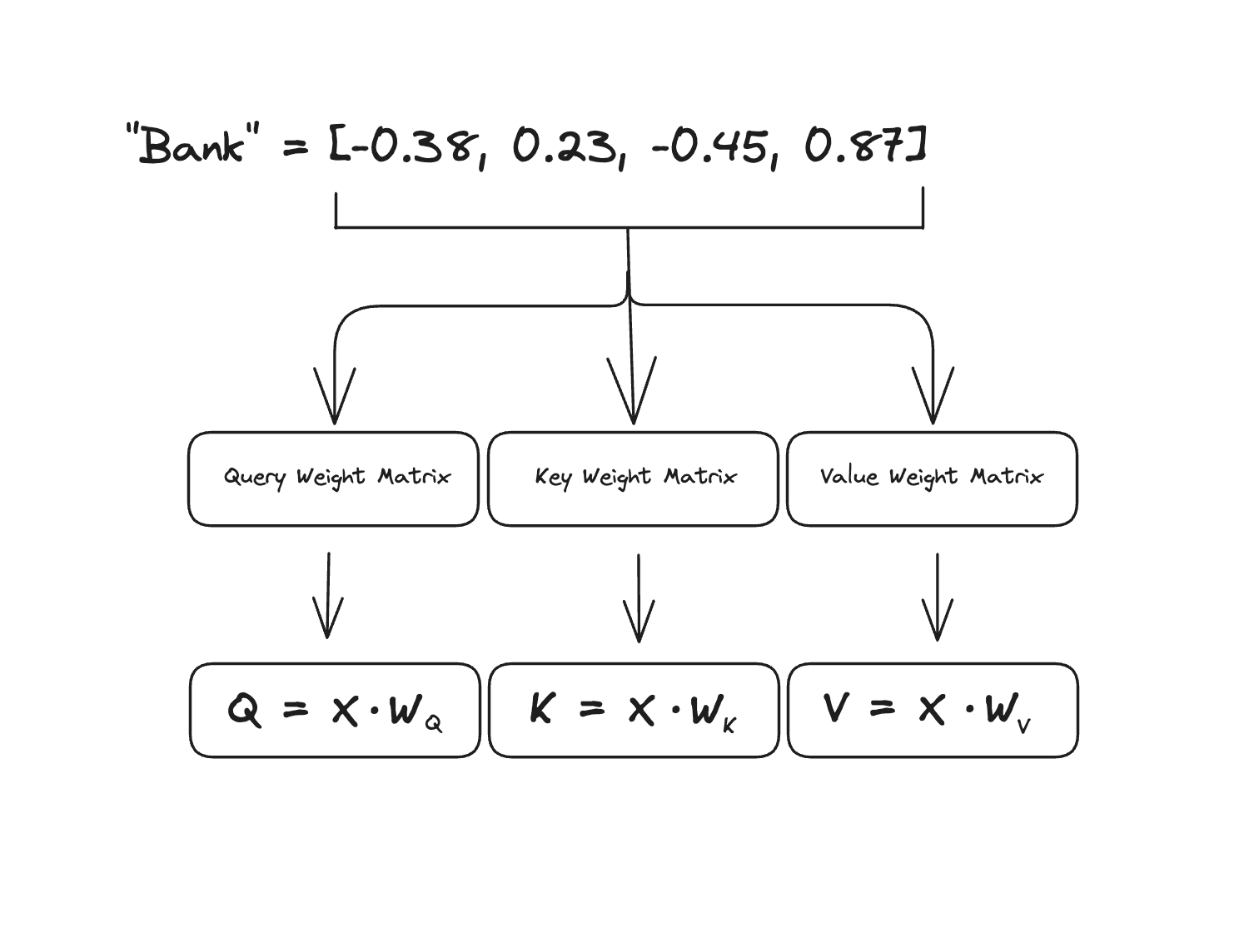
For every word in the sentence, we create three different "views" of that word by multiplying its embedding ( $X$ ) by three different learned weight matrices called the Query, Key and Value matrices.

Using the word "bank" from the example above, we would multiply its embedding by each of the weight matrices like this:

alt

But what do each of these weight matrices represent? Here's the intuition:

Query (Q): Represents what this word is searching for in other words. It encodes what kind of information this token wants to retrieve from others. For example, in the phrase “the cat sat on the mat”, the word “sat” might query for subjects (who sat?), so its query vector looks for noun-like patterns.
Key (K): Represents what this word offers to other words. The key is like a descriptor tag that advertises what kind of information a token carries. In the same example as above, “cat”’s key might encode “noun / animal / subject,” so when “sat”’s query compares itself to “cat”’s key (via a dot product), they match strongly.
Value (V): Represents the actual information this word will contribute when selected. You can think of it as the payload or content that gets passed forward after the attention weights are applied.

Another way to think about it is using a database analogy.

You type Query terms into a search bar ("machine learning papers")
The database checks these against Key indices/tags on each document
When there's a match, you retrieve the Value, the actual document content

In attention, every word is simultaneously:

Searching for relevant information in every other word (via its Query)
Advertising what it contains to every other word (via its Key)
Ready to share its information to every other word (via its Value)

Step-by-Step: How Attention Works

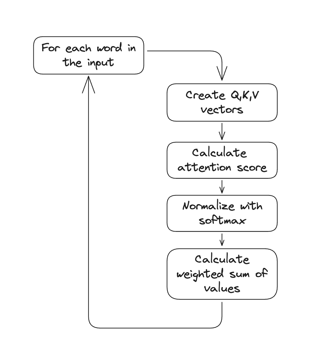
Let's walk through a complete example with the sentence "the cat sat on the mat". Here is the general sequence of steps:

alt

Each word starts with an embedding vector (we'll use 4 dimensions to keep it simple):

the = [0.5, 0.8, 0.1, 0.3]
cat = [1.0, 0.2, 0.5, 0.1]
sat = [0.3, 1.0, 0.2, 0.4]
on  = [0.6, 0.4, 0.7, 0.5]
the = [0.5, 0.8, 0.1, 0.3]
mat = [0.8, 0.1, 0.9, 0.2]

Step 1: Create Q, K, V for Each Word

We multiply each embedding by three weight matrices. Let's assume our learned weight matrices are (4×3 to project to 3D for simplicity):

W_Q = \begin{bmatrix} 0.2 & 0.1 & 0.3 \\ 0.4 & 0.2 & 0.1 \\ 0.1 & 0.5 & 0.2 \\ 0.3 & 0.1 & 0.4 \end{bmatrix}, \quad W_K = \begin{bmatrix} 0.3 & 0.2 & 0.1 \\ 0.1 & 0.4 & 0.3 \\ 0.2 & 0.1 & 0.5 \\ 0.4 & 0.3 & 0.2 \end{bmatrix}, \quad W_V = \begin{bmatrix} 0.1 & 0.3 & 0.2 \\ 0.2 & 0.1 & 0.4 \\ 0.5 & 0.2 & 0.1 \\ 0.3 & 0.4 & 0.3 \end{bmatrix}

If you remember from the "From Matmul to Meaning" blog, multiplying a vector with a matrix returns a vector. Let's do "cat" as an example:
$Q_\text{cat} = [1.0, 0.2, 0.5, 0.1] \cdot W_Q = [0.36, 0.28, 0.39]$
$K_\text{cat} = [1.0, 0.2, 0.5, 0.1] \cdot W_K = [0.46, 0.33, 0.36]$
$V_\text{cat} = [1.0, 0.2, 0.5, 0.1] \cdot W_V = [0.42, 0.45, 0.41]$

After computing Q, K, V for all words, we have:

Queries (Q):               Keys (K):                Values (V):
Q_the = [0.30, 0.35, 0.23]  K_the = [0.34, 0.41, 0.28]  V_the = [0.38, 0.43, 0.32]
Q_cat = [0.36, 0.28, 0.39]  K_cat = [0.46, 0.33, 0.36]  V_cat = [0.42, 0.45, 0.41]
Q_sat = [0.26, 0.44, 0.29]  K_sat = [0.29, 0.52, 0.38]  V_sat = [0.35, 0.38, 0.48]
Q_on  = [0.33, 0.40, 0.35]  K_on  = [0.41, 0.45, 0.42]  V_on  = [0.48, 0.41, 0.39]
Q_the = [0.30, 0.35, 0.23]  K_the = [0.34, 0.41, 0.28]  V_the = [0.38, 0.43, 0.32]
Q_mat = [0.31, 0.38, 0.44]  K_mat = [0.37, 0.34, 0.51]  V_mat = [0.51, 0.49, 0.37]

Step 2: Calculate Attention Scores

Now that we have all of our Q,K,V for every word, we will calculate our attention scores. Attentions scores are calculated by taking the dot product betwee the Q and K vectors of each word.

Why do we take the dot product between Q and K vectors? Remember that the Q vector represents what kind of information this token is searching for, and the K vector represents what information this word offers. So we have a search query and potential matches — we just need to see how well they align. That's where the dot product comes into play.

The dot product measures similarity between vectors: when two vectors point in similar directions (representing similar semantic content), their dot product is large. When they point in different directions, the dot product is small. A high dot product = high similarity = high relevance = this word should pay more attention here.

Let's focus on the word "mat" (last word). Its query $Q_\text{mat} = [0.31, 0.38, 0.44]$ is compared against all keys using dot products:

$\text{score}_\text{mat,the} = Q_\text{mat} \cdot K_\text{the}^T = 0.31 \times 0.34 + 0.38 \times 0.41 + 0.44 \times 0.28 = 0.38$
$\text{score}_\text{mat,cat} = Q_\text{mat} \cdot K_\text{cat}^T = 0.31 \times 0.46 + 0.38 \times 0.33 + 0.44 \times 0.36 = 0.43$
$\text{score}_\text{mat,sat} = Q_\text{mat} \cdot K_\text{sat}^T = 0.31 \times 0.29 + 0.38 \times 0.52 + 0.44 \times 0.38 = 0.45$
$\text{score}_\text{mat,on} = Q_\text{mat} \cdot K_\text{on}^T = 0.31 \times 0.41 + 0.38 \times 0.45 + 0.44 \times 0.42 = 0.49$
$\text{score}_\text{mat,the} = Q_\text{mat} \cdot K_\text{the}^T = 0.31 \times 0.34 + 0.38 \times 0.41 + 0.44 \times 0.28 = 0.38$
$\text{score}_\text{mat,mat} = Q_\text{mat} \cdot K_\text{mat}^T = 0.31 \times 0.37 + 0.38 \times 0.34 + 0.44 \times 0.51 = 0.57$

Raw scores: [0.38, 0.43, 0.45, 0.49, 0.38, 0.57]

Notice that "mat" has the highest attention to itself (0.57) and to nearby contextual words like "on" (0.49). High dot product = high similarity = high relevance.

Also, notice that $Q_\text{mat}$ and $K_\text{mat}^T$ are different despite starting from the same base embedding. This is because each weight matrix (Q,K,V) is different so when you multiply the same embedding by different matrices you get a different output vector.

Next we apply softmax to turn these scores into probabilities that sum to 1:

$\text{attention}_\text{mat} = \text{softmax}([0.38, 0.43, 0.45, 0.49, 0.38, 0.57])$

After softmax: [0.12, 0.14, 0.15, 0.16, 0.12, 0.18]

Why do we turn these into probabilities using softmax? Why not just use the raw attention scores? This is a good question.

Softmax does two critical things:

Normalization: It forces all the attention weights to sum to 1.0 (100%). This means we're creating a proper weighted average, we can't "over-attend" by having weights that sum to more than 100%, and we ensure every word contributes proportionally.
Amplifies differences: Softmax is exponential, which means it amplifies differences between scores. If one word has a score of 0.57 and another has 0.38, softmax makes this difference even more pronounced in the final weights (0.18 vs 0.12). This helps the model make clearer decisions about what to attend to.

Without softmax, using raw scores would cause problems:

The scores could sum to any arbitrary number making it unclear how much to attend to each word proportionally
Small differences in relevance wouldn't be emphasized enough
Training would be less stable because the scale of attention weights would vary wildly across different examples

Back to our example, this means "mat" will:

Pay 12% attention to "the" (first)
Pay 14% attention to "cat"
Pay 15% attention to "sat"
Pay 16% attention to "on"
Pay 12% attention to "the" (second)
Pay 18% attention to itself

These weights sum to approximately 1.0 (100%) giving us nice, proportional weights to work with.

Step 3: Weighted Sum of Values

Now we create a new contextualized representation of "mat" as a weighted combination of all value vectors multipled by the probabilities that we calculated above:

$\text{output}_\text{mat} = 0.12 \cdot V_\text{the} + 0.14 \cdot V_\text{cat} + 0.15 \cdot V_\text{sat} + 0.16 \cdot V_\text{on} + 0.12 \cdot V_\text{the} + 0.18 \cdot V_\text{mat}$

Substituting our value vectors:
$\text{output}_\text{mat} = 0.12 \cdot [0.38, 0.43, 0.32] + 0.14 \cdot [0.42, 0.45, 0.41] + \ldots$

$\text{output}_\text{mat} = [0.45, 0.44, 0.38]$

This is the new contextualized representation of "mat" that incorporates information from the entire sentence, especially from "on" and itself, creating a representation that understands "mat" in the context of being something a cat sat on!

Next, we just repeat this same process simultaneously for all words

"the" (first) attends mostly to "cat" (the noun it modifies)
"cat" attends to "the" (its determiner) and "sat" (its action)
"sat" attends to "cat" (the subject) and "mat" (the object via "on")
"on" attends to "sat" (the verb) and "mat" (the object it relates)
"the" (second) attends to "mat" (the noun it modifies)
"mat" attends to "on" and itself (as we computed above)

Each word gets a new representation that captures its meaning in the context of the sentence.

If you've ever heard of a KV cache, this is where it comes into play. When generating text token-by-token (like ChatGPT does), the model has already computed the K and V vectors for all previous tokens. Rather than recomputing them from scratch for every new token, we can cache and reuse them.

So if you've generated 100 tokens, and you're generating token 101, you don't need to recompute the Q, K, V vectors for tokens 1-100. You only compute Q, K, V for the new token, then compute attention scores between the new Q and all the cached K vectors, and finally combine the cached V vectors.

This optimization makes generation dramatically faster. Instead of doing O(n²) computations for each new token (where n is sequence length), we only do O(n) computations (because we only have to generate attention scores for just the new token instead of every token with every other token). For a 1000-token conversation, this means ~1000x speedup per token generated!

The problem is that KV caches consume a lot of memory (storing K and V for every token at every layer) which is why we have limits on context windows.

Why This Solves the Context Problem

Remember our "it" problem from one of the earlier sections?

"The animal didn't cross the street because it was too tired."

When attention processes "it":

Its query asks: "What noun am I referring to?"
Compares against keys from "animal" and "street"
"animal" + "tired" have high similarity = high attention score
Pulls in the value vector from "animal"
Now "it" has a representation similar to "animal"

For the other sentence:

"The animal didn't cross the street because it was too wide."

Same process, but:

"street" + "wide" have high similarity → high attention score
"it" pulls in the value vector from "street"
Now "it" has a representation similar to "street"!

The same word gets different representations based on context, all through learned matrix multiplications.

From One Layer to 96 Layers

ChatGPT doesn't use just one attention layer, it uses 96 layers stacked on top of each other. Each layer refines representations in increasingly abstract ways.

Some research on transformer interpretability suggests that earlier layers learn syntax, middle layers learn reasoning and the later layers learn generation. The boundaries are fuzzy and layers don't neatly separate into distinct functions:

alt

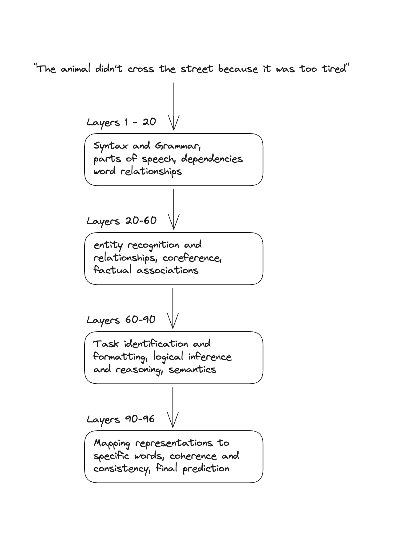
This is still a work in progress but the general trend has been observed across many transformer models.

Wrapping up

There we have it. Attention. It's the mechanism that transformed LLMs from pattern matchers into systems that genuinely understand context.

The word "it" learns to attend to "animal" or "street" depending on context. The word "bank" learns to attend to "river" or "money" depending on its surroundings. Every word dynamically constructs its meaning from every other word.

Attention doesn't just process words sequentially like older models did. It lets every word "see" every other word, compute what matters, and pull in exactly the information it needs. That's what makes LLMs feel human — they understand that meaning doesn't live in individual words, but in the relationships between them.

Evis