In my last post, From Matmul to Meaning, I explained how matrix multiplication is the fundamental operation that lets LLMs understand meaning. We saw how billions of matmuls transform word vectors through semantic space until they produce coherent responses.

At the end of that post, I mentioned that I didn't cover activation functions (mainly because the blog was already getting long) but without activation functions, matrix multiplication can't learn anything interesting.

Even a 96-layer LLM like GPT-4 would collapse into a single matrix multiplication. Wait, what? How can 96 layers of matmul transformations collapse into one?

Let's start at the beginning and build our way to the intuition.

The Problem With Matmul

Let's say we have a simple 2-layer neural network.

h_1 = x \cdot W_1

\hat{y} = h_1 \cdot W_2

Where $x$ is our input (our vector), $W_1$ and $W_2$ are weight matrices, and $h_1$ is the hidden layer and $\hat{y}$ is the output layer.

Visually, this looks like:

alt

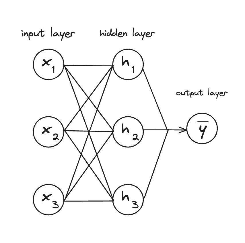
The weights in this diagram are the connections (lines) between nodes. The lines from the input to the hidden layer represent the W₁ matrix, and the lines from hidden to output represent the W₂ matrix. Each line is one weight value, and together they form the complete weight matrices.

We can represent this matrix like this:

W_1 = \begin{bmatrix} w_{x_1 h_1} & w_{x_1 h_2} & w_{x_1 h_3} \\ w_{x_2 h_1} & w_{x_2 h_2} & w_{x_2 h_3} \\ w_{x_3 h_1} & w_{x_3 h_2} & w_{x_3 h_3} \end{bmatrix}, \quad W_2 = \begin{bmatrix} w_{h_1 \hat{y}} \\ w_{h_2 \hat{y}} \\ w_{h_3 \hat{y}} \end{bmatrix}

Where the $w_{x_1 h_1}$ represents the weight going from the ${x_1}$ node to the ${h_1}$ node.

We can simplify our matrices above by substituting the first equation into the second (reading from left to right):

\hat{y} = (x \cdot W_1) \cdot W_2 = x \cdot (W_1 \cdot W_2)

We know that we can easily multiply two matrices together and get a single resulting matrix, so we can combine $W_1 \cdot W_2$ into a single matrix $W$ :

\hat{y} = x \cdot W

Our "2-layer" network just collapsed into a single matrix multiplication!

Let's do this with actual numbers to really drive the point home. Suppose:

x = [1, 2], \quad W_1 = \begin{bmatrix} 2 & 1 \\ 1 & 3 \end{bmatrix}, \quad W_2 = \begin{bmatrix} 1 & 2 \\ 2 & 1 \end{bmatrix}

Layer 1:

h_1 = [1, 2] \cdot \begin{bmatrix} 2 & 1 \\ 1 & 3 \end{bmatrix} = [4, 7]

Layer 2:

\hat{y} = [4, 7] \cdot \begin{bmatrix} 1 & 2 \\ 2 & 1 \end{bmatrix} = [18, 15]

Now let's compute $W_1 \cdot W_2$ directly:

W = W_1 \cdot W_2 = \begin{bmatrix} 2 & 1 \\ 1 & 3 \end{bmatrix} \cdot \begin{bmatrix} 1 & 2 \\ 2 & 1 \end{bmatrix} = \begin{bmatrix} 4 & 5 \\ 7 & 5 \end{bmatrix}

Single layer:

\hat{y} = [1, 2] \cdot \begin{bmatrix} 4 & 5 \\ 7 & 5 \end{bmatrix} = [18, 15]

Same answer!

This is called linearity, and it holds true for any number of layers in a neural network that are purely doing matrix multiplication. No matter how many layers you stack, pure matrix multiplication can only represent linear transformations: rotations, scalings, and shears.

Okay, so layer collapse is bad. But why? But why aren't linear transformations enough?

Why Matmul Isn't Enough

Remember our "king - man + woman = queen" example from the previous blog post? If not, no worries. Let's say we have a simple 2D "word space" where:

The first dimension represents royalty (0 = common, 1 = royal)
The second dimension represents femininity (0 = masculine, 1 = feminine)

So our mini vocabulary looks like this:

Word	Vector (royalty, femininity)
king	[0.9, 0.1]
queen	[0.9, 0.9]
man	[0.1, 0.1]
woman	[0.1, 0.9]

To get from "king" to "queen", we can do some simple vector math:

\text{king} - \text{man} + \text{woman} = [0.9, 0.1] - [0.1, 0.1] + [0.1, 0.9] = [0.9, 0.9] = \text{queen}

This works because it was a linear operation in vector space. This is linear because:

We know: king → [0.9, 0.1], man → [0.1, 0.1], woman → [0.1, 0.9]
We can predict: king - man + woman → [0.9, 0.1] - [0.1, 0.1] + [0.1, 0.9] = [0.9, 0.9]

The result is exactly the sum of the individual transformations. That's what makes it linear.

But language is complex and rarely linear.

"Bank" means different things near "river" vs "money"
"Not bad" means "good" (negation reverses sentiment)
"The animal didn't cross because it was tired" requires reasoning

Linear transformations can't capture this complexity. You need something that can learn the curves, corners, and complex decision boundaries that comes with modeling language in a higher dimensional space.

So how do we create this non-linearity? Simple - we use a non-linear function!

Non-Linear Functions?

But what is a non-linear function? Let's approach it from the other side. What is a linear function?

A function $f$ is linear if it satisfies two properties:

Additivity: $f(x + y) = f(x) + f(y)$
Homogeneity: $f(a \cdot x) = a \cdot f(x)$

Matrix multiplication is linear because it satisfies both:

$(x + y) \cdot W = x \cdot W + y \cdot W$
$(a \cdot x) \cdot W = a \cdot (x \cdot W)$

We saw this in the first section where we could our two weight matrices into one. A function is non-linear if it breaks at least one of these properties.

Let's look at a simple non-linear function: $f(x) = x^2$

Test additivity:

f(2 + 3) = 5^2 = 25

f(2) + f(3) = 4 + 9 = 13

25 \neq 13 \text{ ✗}

Since this test fails, this function is non-linear!

Breaking Linearity

Now that we have the background context, we can get to activation functions.

An activation function is a non-linear function applied element-wise to the output of each layer. Remember that when we multiply an input vector by a matrix, we get another vector as output. "Element-wise" means we apply the activation function to each element in that output vector individually.

For example, if our layer outputs the vector [2, -1, 3], and our activation function is $\sigma$ , we compute:

\sigma([2, -1, 3]) = [\sigma(2), \sigma(-1), \sigma(3)]

Each element gets transformed independently by the same function. Okay, that makes sense, but how does an activation function break linearity?

In the top section, we combined our two equations and got:

\hat{y} = (x \cdot W_1) \cdot W_2

Since matrix multiplication is associative (you can regroup: $(A \cdot B) \cdot C = A \cdot (B \cdot C)$ ), we can merge multiple matrices into one.

Now let's insert a non-linear function $\sigma$ (the activation):

h_1 = \sigma(x \cdot W_1)

\hat{y} = \sigma(h_1 \cdot W_2)

Now we're stuck. We can't collapse this into a single matrix because the activation is in the way:

\sigma(\sigma(x \cdot W_1) \cdot W_2) \neq \sigma(x \cdot W_{\text{combined}})

But, why not? This gets at the heart of linear algebra. In linear algebra, Matrix multiplication is linear, so it distributes:

(x \cdot W_1) \cdot W_2 = x \cdot (W_1 \cdot W_2)

But activation functions are inherently non-linear, so they don't distribute:

\sigma(A \cdot B) \neq \sigma(A) \cdot \sigma(B)

You can't "push" the $\sigma$ through the matrix multiplication or split it up. Once applied, it fundamentally changes the values in a way that can't be undone or rearranged.

Let's look at two of the most common activation functions.

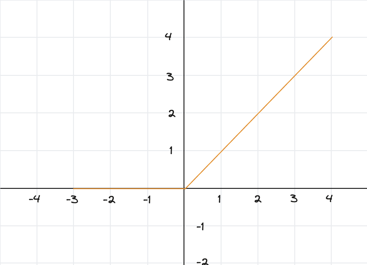
ReLU (Rectified Linear Unit)

The simplest and most popular activation function:

\text{ReLU}(x) = \max(0, x) = \begin{cases} x & \text{if } x > 0 \\ 0 & \text{if } x \leq 0 \end{cases}

ReLU zeros out negative values but keeps positive values unchanged.

For example:

x = [-2, -1, 0, 1, 2]

\text{ReLU}(x) = [0, 0, 0, 1, 2]

Graphically:

alt

Why ReLU works so well:

1. Sparsity

ReLU zeros out negative values. In a typical network, about half the values going through each layer are negative, which means:

About 50% of neurons output zero (they're "off")
The network only computes with the active neurons
This makes the network faster and uses less memory

But wait - wouldn't zero'ing out half of the neurons mean that network doesn't learn as well? Actually, no! When ReLU zeros out a neuron, it's saying: "This feature isn't relevant for this input." That's a decision the network learned to make during training, not a random deletion.

2. Simple gradient

During training, the network needs to calculate derivatives (gradients) to know how to adjust weights (backpropagation). ReLU's derivative is incredibly simple:

Either 1 or 0. That's it!

3. Non-saturating (Doesn't get stuck)

"Saturation" means a function's output stops changing even when the input keeps changing. For example, let's look at Sigmoid activation functions which saturates.

Input: 5 → Output: 0.993
Input: 10 → Output: 0.99995
Input: 100 → Output: 0.9999999...

The output is stuck near 1, barely moving. This means the gradient (how much to adjust weights) becomes nearly zero, so learning stops. This is called the vanishing gradient problem.

ReLU (doesn't saturate for positive values):

Input: 5 → Output: 5
Input: 10 → Output: 10
Input: 100 → Output: 100

The output keeps growing! The gradient stays at 1, so learning never slows down. This is huge for training deep networks where gradients need to flow back through 96+ layers.

ReLU acts like a smart filter that creates selective pathways through the network where only the neurons that found relevant patterns pass information forward.

GELU (Gaussian Error Linear Unit)

A smoother, more sophisticated version of ReLU:

\text{GELU}(x) = x \cdot \Phi(x)

Where $\Phi(x)$ is the cumulative distribution function of the standard normal distribution. In practice, it's approximated as:

\text{GELU}(x) \approx 0.5x \left(1 + \tanh\left[\sqrt{\frac{2}{\pi}} \left(x + 0.044715x^3\right)\right]\right)

For example:

x = [-2, -1, 0, 1, 2]

\text{GELU}(x) \approx [-0.04, -0.16, 0, 0.84, 1.96]

Graphically:

alt

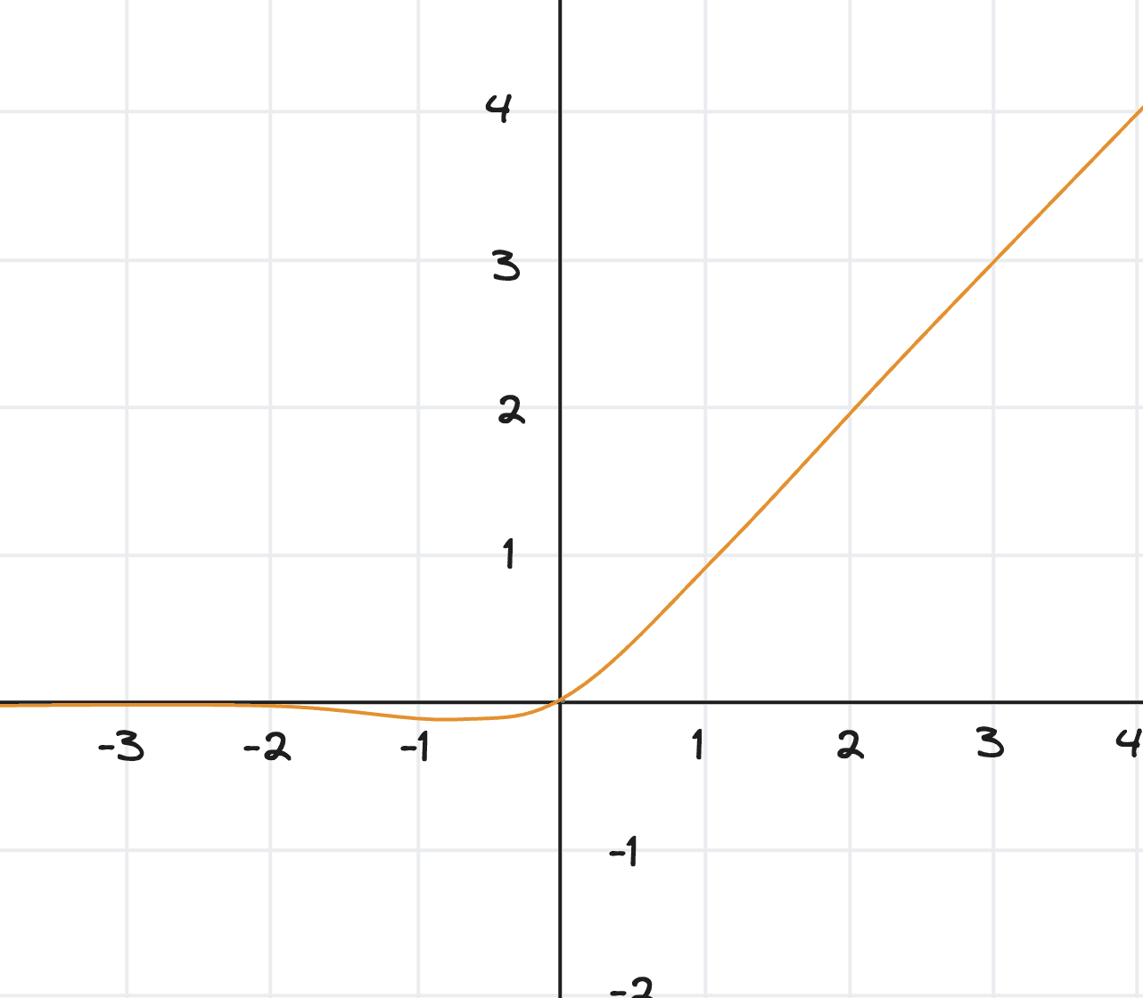
What it does: Similar to ReLU but with smooth transitions instead of a hard cutoff at zero.

Notice that small negative values get small negative outputs (not zero like ReLU). This "soft gating" preserves more information.

Why it works:

Smooth gradients: Better for optimization (no sudden jumps)
Probabilistic interpretation: It's like asking "what's the probability this neuron should be active?"
Better performance: Empirically outperforms ReLU on large language models

ELU is like a probabilistic gate. Instead of a hard on/off switch, it asks "how confident am I that this feature is relevant?" and scales the output accordingly.

Modern LLMs like GPT-3, GPT-4, and LLaMA all use GELU or variants of it. The smooth gradients help with training stability at massive scale.

Learning with Activation Functions

Now that we've developed some intuition about activation functions, let's see an example of how activations let us learn non-linear patterns.

Suppose we want to learn the XOR function (exclusive or):

Input ( $x_1$ , $x_2$ )	Output
(0, 0)	0 (blue)
(0, 1)	1 (red)
(1, 0)	1 (red)
(1, 1)	0 (blue)

alt

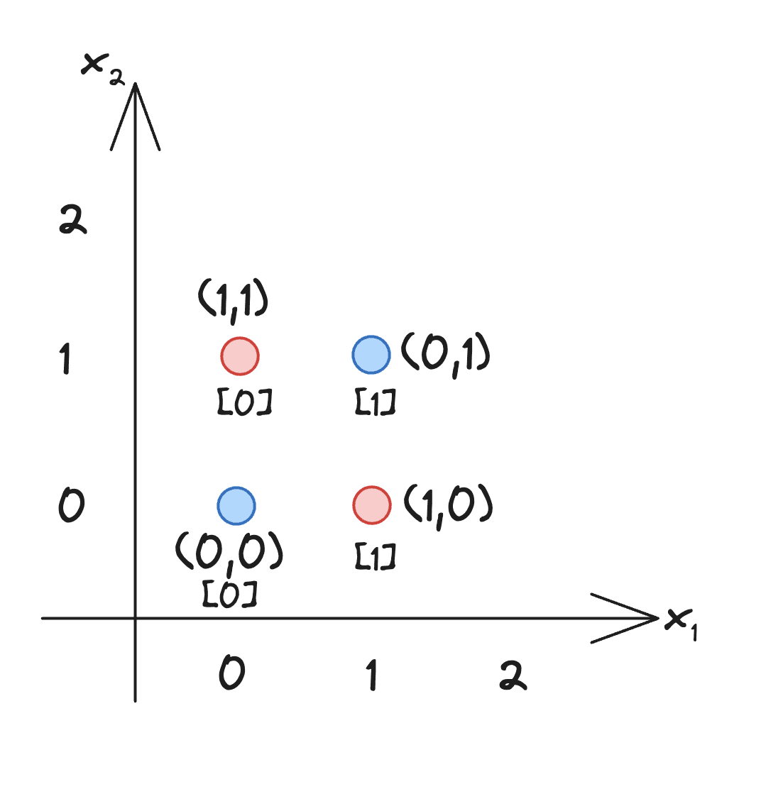
This is the classic example of a non-linearly separable function. You can't draw a single straight line to separate the 1s from the 0s. This is what we saw in the "Breaking Linearity" section. No matter what weight matrix $W$ you use, $y = x \cdot W$ can't solve XOR. It can only produce linear decision boundaries.

Now let's use activations.

Great question! Let me explain what's happening with the XOR example more clearly:

Let's use a 2-layer network with ReLU to solve XOR:

h = \text{ReLU}(x \cdot W_1)

\hat{y} = h \cdot W_2

With learned weights:

W_1 = \begin{bmatrix} 1 & 1 \\ 1 & 1 \end{bmatrix}, \quad W_2 = \begin{bmatrix} 1 \\ -2 \end{bmatrix}

Let's trace through all four XOR inputs to see the pattern:

The $^T$ superscript that you'll see below (like, $[1, -2]^T$ ) is a shorthand
marker that means to transpose the matrix. You transpose a matrix by
switching the rows and columns. For example, if you have a row vector $[1, -2]$ , and you transpose it, you get a column vector $\begin{bmatrix} 1 \\ -2 \end{bmatrix}$ .

Input (0, 0) → Should output 0:

Layer 1: $h = \text{ReLU}([0,0] \cdot W_1) = \text{ReLU}([0,0]) = [0,0]$
Layer 2: $\hat{y} = [0,0] \cdot [1, -2]^T = 0$

Input (0, 1) → Should output 1:

Layer 1: $h = \text{ReLU}([0,1] \cdot W_1) = \text{ReLU}([1,1]) = [1,1]$
Layer 2: $\hat{y} = [1,1] \cdot [1, -2]^T = 1 - 2 = -1 \approx$ 1 (after threshold)

Input (1, 0) → Should output 1:

Layer 1: $h = \text{ReLU}([1,0] \cdot W_1) = \text{ReLU}([1,1]) = [1,1]$
Layer 2: $\hat{y} = [1,1] \cdot [1, -2]^T = -1 \approx$ 1

Input (1, 1) → Should output 0:

Layer 1: $h = \text{ReLU}([1,1] \cdot W_1) = \text{ReLU}([2,2]) = [2,2]$
Layer 2: $\hat{y} = [2,2] \cdot [1, -2]^T = 2 - 4 = -2 \approx$ 0

What created the non-linear boundary?

The ReLU in Layer 1 transformed the input space. Here's what happened:

Inputs (0,1) and (1,0) both became [1,1] after ReLU
Input (1,1) became [2,2] - different from the others
Input (0,0) stayed [0,0]

Visually:

alt

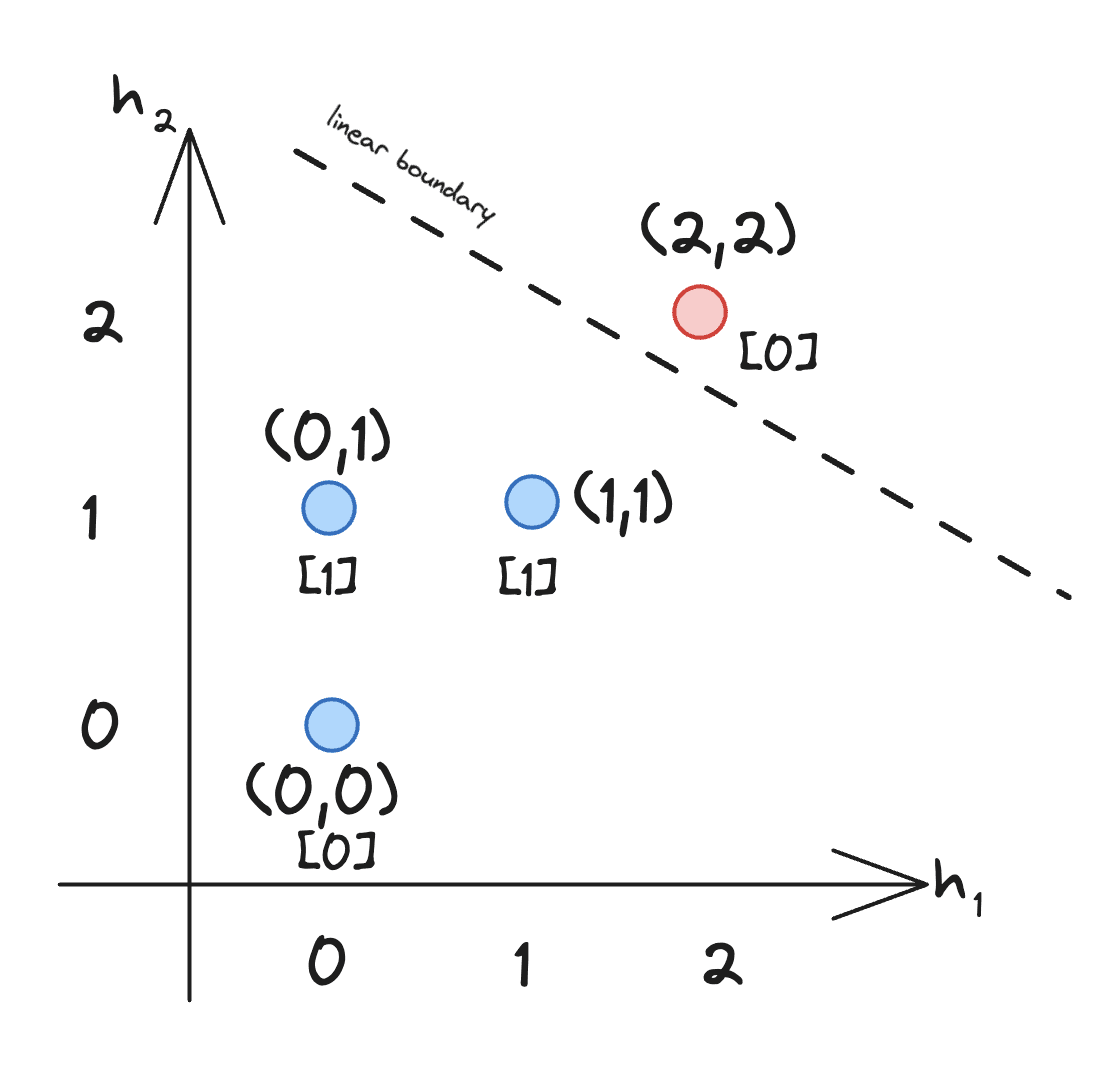
The ReLU created a new space (the hidden layer) where Layer 2 can draw a simple linear boundary to separate XOR! But it required transforming the feature space first using the activation function.

The key insight is that ReLU and other activations functions allow you to transform the feature space, bending and warping it like a sheet of paper so that XOR becomes linearly separable in the new space.

From XOR to Language Understanding

The XOR example seems pretty basic, but the principle scales to language as well.

Consider understanding negation (we saw an example of this above): "not good" vs "not bad"

"good" → positive sentiment
"not good" → negative sentiment
"bad" → negative sentiment
"not bad" → positive sentiment (!)

This is non-linear! The word "not" doesn't just shift sentiment by a fixed amount (if we were to do vector arithmetic), it reverses it based on context.

Here's an example of how a neural net could learn the nuances of language layer by layer using activations:

Layer 1-20: Learn that "not" is a modifier
Layer 21-40: Learn that "not" near sentiment words reverses polarity
Layer 41-60: Learn that "not bad" is idiomatic (means "good", not just "not negative")
Layer 61-80: Learn when this pattern applies vs when "not bad" means "terrible"

The activation functions at each layer creates a new feature space where these increasingly complex patterns become learnable via linear transformations.

Why Not Just Use One Big Activation?

Why do we need to use activation functions are every layer? Why not just use one activation function? Something like:

y = \sigma(x \cdot W_1 \cdot W_2 \cdot W_3 \cdot ... \cdot W_{96})

Because then you're back to a single linear transformation! Remember, all those matmuls collapse:

y = \sigma(x \cdot W_{\text{combined}})

So you end up getting just a single non-linear transformation. It's slightly better than pure linear, but nowhere near as expressive as 96 layers of matmul + activation functions.

Each activation functions creates a new opportunity to reshape the feature space in order to find that boundary. With 96 activations, you get 96 chances to create increasingly abstract representations.

The Universal Approximation Theorem

Hopefully by now you have a good understanding of activation functions and why they are so important in neural networks so let's take a quick detour into history.

In 1989, a mathematician named George Cybenko proved something amazing. He showed that a neural network with:

At least one hidden layer where each neuron applies a non-linear activation function (we'll get into this so don't worry if you don't know what it means)
Enough neurons

Can approximate any continuous function to arbitrary precision. This means that neural networks with activation functions are theoretically powerful enough to learn any pattern in data, whether that's recognizing faces, translating languages, or predicting the next word in a sentence.

The key that makes this work is the activation function. Without it, your neural net layers end up collapsing (as we saw). But with the activation functions, you can stack 96 layers of transformations, each one a linear projection (matmul) followed by a non-linear activation, and your neural net will build a function so complex that it can have a human-like conversation.

With enough depth and non-linearity, you can approximate anything.

Wrapping Up

Matrix multiplication gives us efficient, learnable transformations. But it's activations that let those transformations build on each other, creating the hierarchical, non-linear feature extraction that makes modern AI possible.

Each matmul rotates and scales the feature space.
Each activation reshapes it non-linearly.
Do this 96 times, and you get something that can understand and generate human language.

Pretty wild that $\max(0, x)$ is part of what makes ChatGPT possible ...

Until next time!

Evis