How do LLMs like ChatGPT or Claude learn? What's actually happening inside ChatGPT or Claude as it's learning? What does it even mean for an LLM to "learn"?

When I first started learning about LLMs, I found myself coming back to these questions over and over again, trying to paint a clear picture in my head of how a neural net goes from multiplying numbers to writing code. What I eventually discovered is that the underlying mechanics are surprisingly elegant once you see how all the pieces connect.

Eventually it clicked and I got so excited that I wanted to write a technical yet intuitive guide that answers these questions from first principles. Something that could have guided my understanding in the beginning.

We'll walk through how loss functions, gradient descent, and optimizers work together to update model weights and help neural nets learn.

We'll cover the math, but more importantly, we'll build the intuition of why it all works.

Let's jump in.

The Optimization Problem

Think about the last time that you learned something new. Maybe it was a new skill or recipe. Your first attempt? Probably not perfect. But each time you try again, you get a little closer. You think about what you need to do, make adjustments, tweak the timing and eventually you nail it.

Neural networks learn in a similar way. We can train a neural network to learn how to classify an email as spam or predict the next token, and over a number of repititions (we call them epochs), they gradually improve until we're happy with the results (or it doesn't, and we're back to square one).

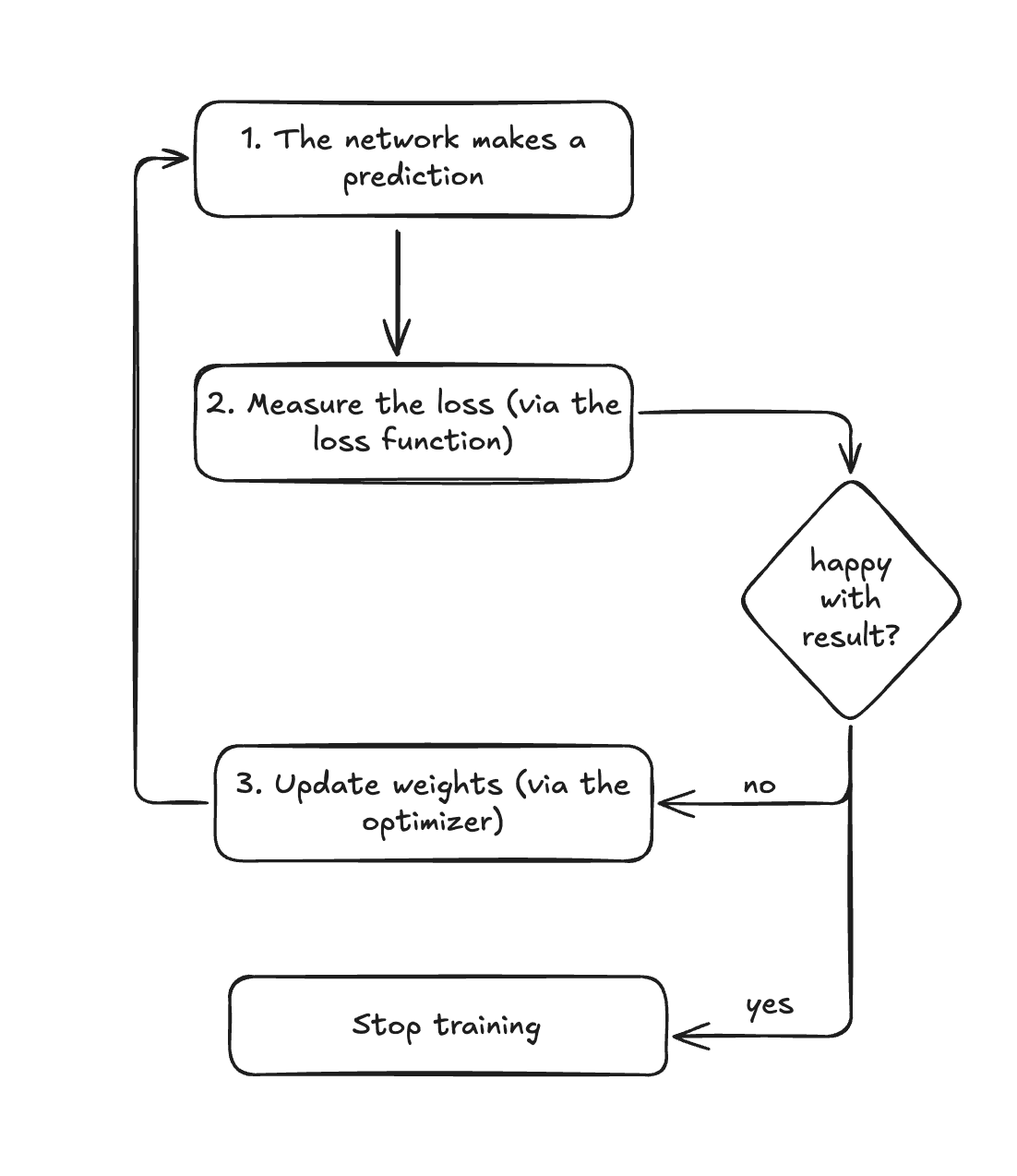
We can generally describe this process:

1. The network makes a prediction
2. We measure how far off it was from the correct answer, if we're happy then we stop training, otherwise, we continue
3. The neural network adjusts its internal parameters to hopefully do better next time
4. Repeat step 1

The success of this process relies on two fundamental concepts:

1. Measuring how far off we are from where we want to be. We call this measure a loss function. The goal is to make this distance as small as possible so we are as close to our ideal state as possible. In the email spam example above, this would mean being able to perfectly classify every spam email as spam and never missing one. In reality, we're never perfect but we try to get as close as we can.

2. Updating our model weights to reduce the loss function next time we try again. This is done by an algorithm called an optimizer. Optimizers decide how to adjust weights in order to reduce the loss.

So our loss function tells us how far off our prediction is from the correct answer and our optimzier helps us update the weights in the neural network so we can try again and hopefully be closer.

Said differently, at its core, training a neural network is an optimization problem. We have a loss function, let's call it: $L(θ)$ that measures how wrong our model is, and we want to find parameters (weights) $θ$ that minimize this loss which ultimately produces a more accurate (and ideally precise) model.

But, first, how do we measure the loss?

How Wrong Are We?

The loss function tells us how far our model's predictions are from the truth. But how do we know what the truth is?

Training with Answers

In supervised learning, we train models using labeled data where we already know the correct answer.

Let's look at two examples:

For a spam classifier: We have thousands of emails that humans have already labeled as "spam" or "not spam." The model makes predictions, and we compare them against these known labels. When the model is wrong, our loss increases, indicating that the model needs to update it's weights next time (via the optimizer) and try to reduce the loss on the next epoch.

A decreasing loss over time is good while an increasing loss is bad. With that being said, there is a point of diminishing returns where the loss "converges" (the technical term) where it's leveled off and the model is as good as it's going to be with that set of weights.

For LLMs: The process is actually pretty simple. We train the model on data from the internet, books and other text sources, feeding in batches of tokens (words or parts of words) that represent sentences. Then we test the model by asking it to predict the next token. For example, take the sentence: "ChatGPT can make mistakes."

We train the model by:

1. Feeding in "ChatGPT" → asking it to predict "can"
2. Feeding in "ChatGPT can" → asking it to predict "make"
3. Feeding in "ChatGPT can make" → asking it to predict "mistakes"

This is what we mean by "next-token prediction", it's literally predicting the next token in the sentence.

The next token in the training text is the ground truth. We know what should come next because it's right there in the data - it's the next token.

This is called self-supervised learning because the model generates its own training labels from the structure of the data itself, no humans needed to manually label millions of examples.

Loss Functions

As we're training our models, we're measuring how right or wrong our model was on every prediction and then averaging that together to measure our loss. The loss function is the algorithm that we use to measure how right or wrong our model was on every prediction.

There are different types of loss functions but many LLMs use cross-entropy loss, which is perfect for the next-token prediction task. For each token the model is trying to predict, the model outputs a probability distribution over its entire vocabulary (often 50,000+ possible tokens), and cross-entropy measures how confident it was about the correct next token.

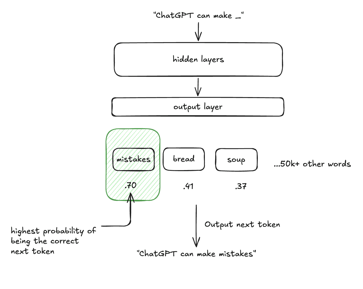
Think of it like a confidence penalty: if your model says "I'm 95% sure the next word is 'mistakes'" and it actually is "mistakes", the loss is very small. But if it says "I'm 95% sure the next word is 'bread'" when it should be "mistakes"? The loss shoots up dramatically.

Mathematically, for each token prediction:

$L = -\log(p_{\text{correct}})$

Where p_correct is the probability the model assigned to the actual next token. So in our example, the .70 or .41 or .37.

If "mistakes" is correct: L = -log(0.70) ≈ 0.357

If "soup" was somehow correct: L = -log(0.37) ≈ 0.994

If we had another word that had a probability of 0.12 then the negative log loss would be 2.120. You can see that the loss starts to really scale if the word that is chosen has a very low probability. The logarithm ensures that being confident and wrong is penalized, while being confident and right is rewarded.

Aggregating Across the Sequence

For a full sentence, we average the loss across all token predictions:

$L = -\frac{1}{n} \sum_{i=1}^{n} \log(p_{\text{correct}_i})$

Where n is the number of tokens and we sum over each prediction in the sequence.

This makes intuitive sense. We're asking the model to predict 5 different tokens. For each token, we see how right or wrong it was (our loss) and then we average that to get a final loss number. If the number is high then our model was often wrong. If it's low, then our model was often right.

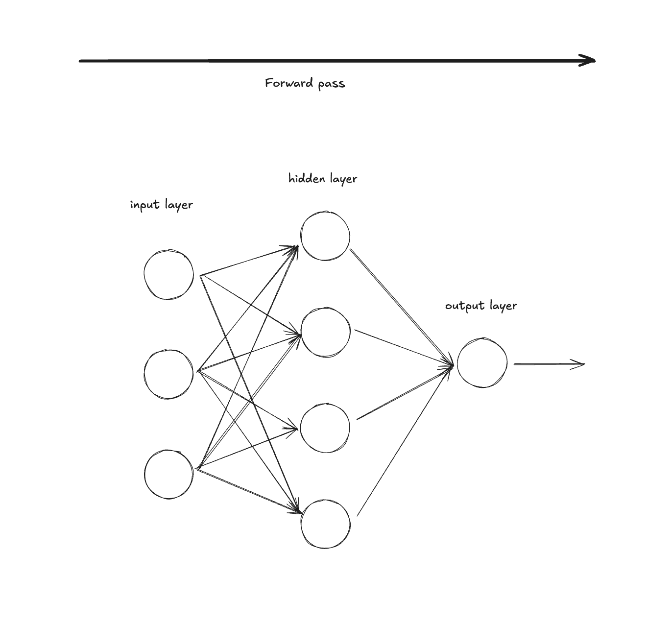
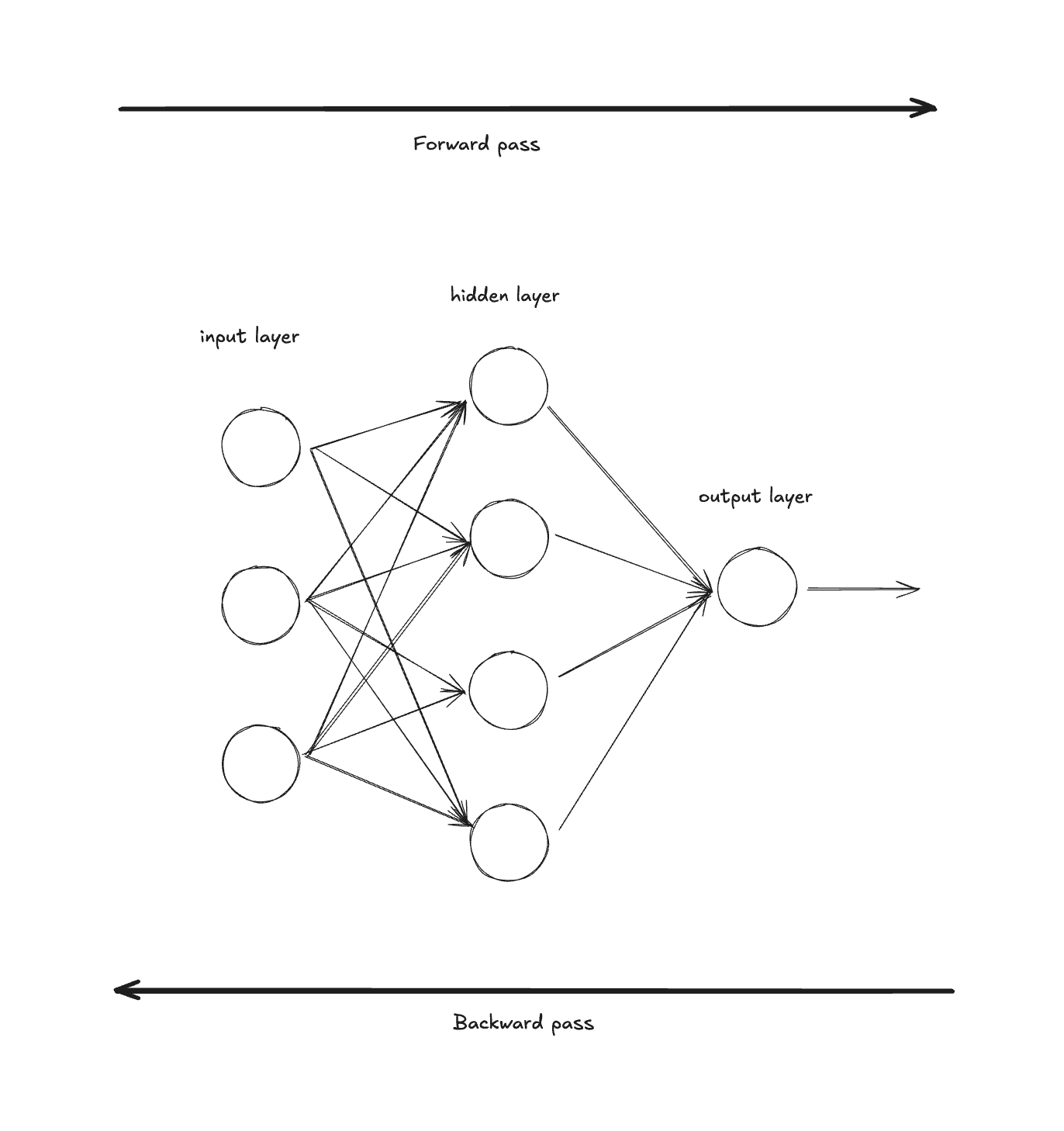
The process of feeding in training data to your model and computing the loss function for every parameter is called the forward pass.

Now that we can measure how right or wrong our predictions are (using the loss), how do we improve our model to get better over time?

Hill Climbing

When we first initialize our model, we do it with random weights (we have to start somewhere and randomly assigning weights is good enough.) We then make our first forward pass (as described above). At the end of that forward pass we have a loss value that is calculated by our loss function. Since we used random weights, our loss function is predictably going to be high and our model is not going to be very accurate.

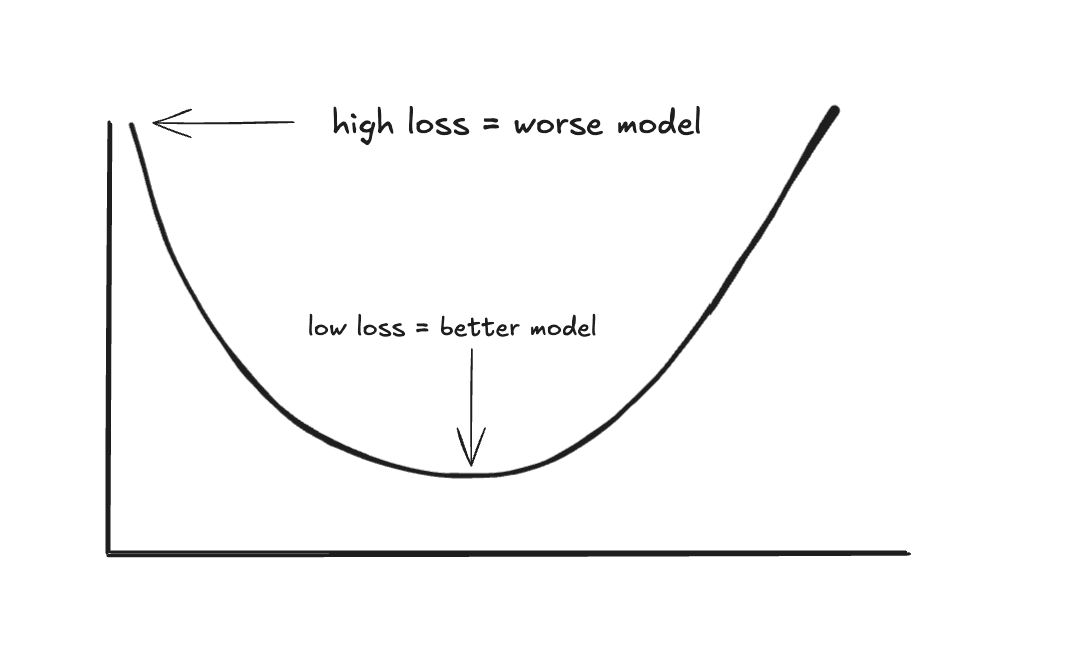
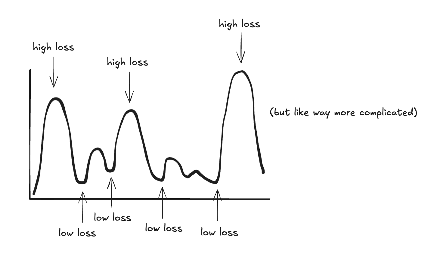
One way to think about loss functions is to imagine it as a hilly landscape where the height at any point represents how wrong (or right) your model is with those particular weights. The lower the point is on a hill or in the landscape, the lower the loss and the better the model.

For simple models, this landscape might be a smooth bowl, there's one obvious lowest point.

But for LLMs with billions of parameters the landscape is extraordinarily complex, with countless hills, valleys, and saddle points in billions of dimensions.

Since we intialize our model with random weights, we might be dropped anywhere on this hilly landscape. Our goal is to reach the lowest points in the landscape (which represents the lowest loss), but there's a twist. Every step we take changes the hilly landscape across the millions or billions of parameters that we have. It might increase the loss for some parameters while decreasing the loss for others.

Then how do we navigate this hilly loss landscape? And how do we do it efficiently if every step we take means updating millions or billions of parameters?

Gradient Descent

Imagine you're blindfolded on the hilly landscape we mentioned above and you can only feel the slope beneath your feet, how do you find the lowest point in the hilly landscape?

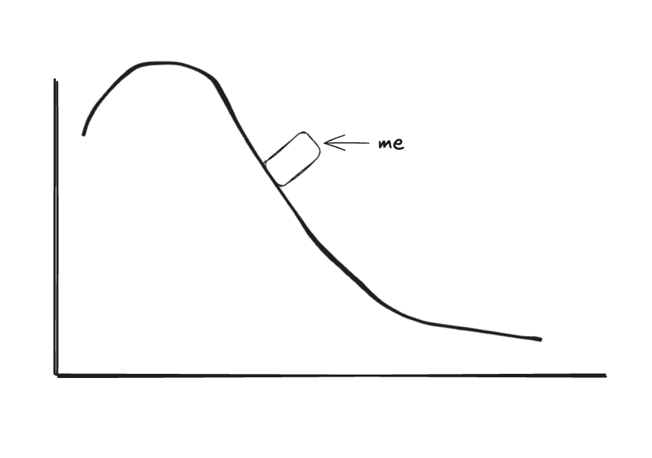
Well if you can feel the slope under your feet, then you can just follow it downward until you get to the bottom. You won't know if that's the lowest point of all of the hills in the entire landscape, but it's surely lower than where you started.

This slope is called the gradient. It tells you which direction slopes downward most steeply.

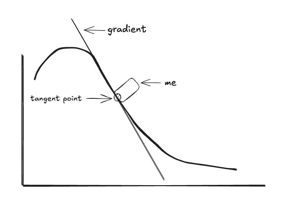
The gradient is the tangent line at any given point on a curve. And the size of the step that you take down the curve, following the gradient, is called the learning rate.

Okay, so we're on a hill and we want to walk down the slope. And if we do that then that will decrease our loss and our model will be more accurate. Great, so we can just take the biggest step that we can so we can reach the bottom as fast as we can, right?

It's unfortunately not that simple. If you take steps that are too large, you might overshoot the valley entirely and end up on the opposite hill! Imagine taking a giant leap while blindfolded - you could fly right past the lowest point and land somewhere even higher than the bottom. Worse yet, you might start bouncing back and forth across the valley, never actually settling at the bottom.

This is why choosing the right learning rate (step size) is crucial. Too small, and you'll take forever to reach the bottom (or get stuck in a shallow dip). Too large, and you'll overshoot.

Finding the right learning rate for is one of the key challenges in training neural networks. Thankfully, there's been a lot of research in this area and, generally speaking, learning rates around 1e-4 are standard for pretraining LLMs.

Okay, now that we've developed the conceptual intuition, let's work through the math step-by-step.

The Math

Mathematically, we define gradient descent as:

$\theta_{t+1} = \theta_t - \alpha \nabla L(\theta_t)$

Where:

• θ_t are the parameters at time step t
• α is the learning rate (step size)
• ∇L(θ_t) is the gradient of the loss with respect to parameters

Let's break down what this equation is actually saying:

θ_t - This is where you currently are on the landscape (your current parameter values for your model)

∇L(θ_t) - This is the direction of steepest ascent at your current position. It points uphill. Think of it as a vector that says "if you go this way, the loss increases most rapidly."

- ∇L(θ_t) - By putting a negative sign in front, we flip the direction to point downhill instead. Now we're pointing toward where the loss decreases most rapidly.

α - This controls how big of a step we take in that downhill direction. A larger α means bigger steps, smaller α means smaller, more cautious steps.

θ_t - α∇L(θ_t) - This is your new position. We take where you were (θ_t) and move in the downhill direction (-∇L) by a distance controlled by the learning rate (α).

θ_{t+1} - This is simply the name for your new position after taking that step.

So the whole equation says: "Your next position equals your current position, minus a step in the steepest downhill direction." We repeat this process over and over, taking small steps downhill until we reach a valley (a minimum in the loss).

This process of computing gradients and updating our parameters happens in what's called the backward pass (also known as backpropagation).

Here's how it works:

• Start with the loss (we calculated this above)
• Work backwards through the model, calculating the gradient for every parameter in the model
• Update all parameters using those gradients

Why is it called "backward pass"? Because we're literally moving in the opposite direction of the forward pass through the network. The forward pass goes input → hidden layers → output. The backward pass goes output → hidden layers → input, computing how much each parameter contributed to the loss.

If you're thinking, "wow that's a lot to process for just one step", then you're exactly right. It is. And it's not the only problem. There are three big problems:

1. Computationally expensive: Computing gradients over the entire dataset is slow. If you have a billion training examples, you need to process all of them before taking a single step.

2. No memory: Each step completely forgets previous steps. If the loss surface is shaped like a narrow valley, you'll bounce back and forth between the walls while making slow progress forward.

3. Fixed learning rate: Same step size everywhere, even when the terrain varies dramatically. Sometimes you're on a gentle slope and could take big steps. Other times you're near the minimum and should take tiny steps.

The good thing is that we can address of each of these problems by making some slight changes to the gradient descent formula that results in big performance gains.

Stochastic Gradient Descent (SGD)

Let's tackle the first problem: computing gradients over the entire dataset is slow.

In normal gradient descent, if we have 1 million examples in our training data, we will process 1 millino examples and then have to calculate gradients for those parameters. That's a lot of calculations to perform for every step we take.

What if we didn't do the entire training dataset at once? What if we batched the dataset into smaller batches and then ran those through the model?

This is the core idea behind Stochastic Gradient Descent (SGD).

We'd still run the same total amount of training data just batched up in small groups. As it turns out, this batching doesn't make the model worse, in fact, it actually makes it more resilient in some ways.

Think of it like polling in an election. You don't need to survey every single voter in the country to understand who's winning, a representative sample of 1,000 people gives you a pretty good estimate. Similarly, a small mini-batch of training examples gives you a noisy but useful estimate of the true gradient.

Imagine you have a million training examples:

• Regular Gradient Descent: You carefully measure all 1 million examples, then take 1 step. Repeat.
• SGD with batch size 32: You quickly measure 32 examples, take a step. You can do this ~31,000 times while gradient descent is still on its first step!

Even though each step is less precise, taking 31,000 noisy steps gets you to the bottom much faster than taking 1 perfect step. In fact, the noise actually helps to regularize the model so that it generalizes better to new data.

The Math

Mathematically, instead of computing gradients over the entire dataset D, we compute them on randomly sampled mini-batches:

$\theta_{t+1} = \theta_t - \alpha \nabla L(\theta_t; \mathcal{B}_t)$

Where:

• $\mathcal{B}_t$ is a mini-batch sampled from your dataset at step t
• Everything else is the same as gradient descent

Let's break down what changed:

In regular gradient descent, we had $\nabla L(\theta_t)$ which meant "compute the gradient using all the data."

Now we have $\nabla L(\theta_t; \mathcal{B}_t)$ which means "compute the gradient using just this mini-batch."

The size of the mini-batch matters:

• Batch size = 1: Pure stochastic gradient descent (very noisy, but extremely fast updates)
• Batch size = 32-256: Common sweet spot for most applications
• Batch size = 1000s: Approaching full gradient descent (less noise, but slower)

In modern LLM training, batch sizes are often quite large (thousands or even millions of tokens) to take advantage of parallel GPU computation, but they're still much smaller than computing over the entire training dataset.

So the equation says: "Your next position equals your current position, minus a step in the downhill direction estimated from a small random sample." We repeat this thousands of times, and even though each step is imperfect, we rapidly converge toward the valley.

Adding Momentum

Now let's move onto the second problem: remembering gradients from past steps to converge faster.

One of the downsides of SGD is that each step is stateless and doesn't remember how we updated previous gradients. This can cause wild swings in gradients that slow down the convergence process.

We can smooth out the learning process by adding in a velocity term into our SGD equation from above:

v_t = γ · v_(t-1) + α · ∇L(θ_t)
θ_(t+1) = θ_t - v_t

Where γ (typically 0.9) is the momentum coefficient.

Expanded recursively:

v_t = α · g_t + γ · α · g_(t-1) + γ² · α · g_(t-2) + γ³ · α · g_(t-3) + ...

This is an exponentially weighted moving average of past gradients, where recent gradients have more influence.

The parameter update now has inertia. Think of a ball rolling downhill:

• If gradients consistently point in the same direction, you build up speed (like rolling down a long slope)
• If they oscillate, the momentum dampens the zigzagging (like friction smoothing out the path)
• You can roll through shallow local minima instead of getting stuck

Why It Works

The γ parameter controls how much history you remember:

• γ = 0: No momentum (regular SGD)—you instantly forget everything
• γ = 0.9: Roughly 10 steps of memory (1/(1-0.9) ≈ 10)
• γ = 0.99: Roughly 100 steps of memory
• γ → 1: Infinite memory—you never slow down

This makes our learning process much smoother and allows us to move fast in places where it makes sense while smoothing out variances.

Adaptive Learning Rates

Lastly, let's move onto the final problem: static learning rates.

Our hilly landscape can have small hills, big hills and some in between. Given that our learning rate represents the size of the step that we're going to take in any direction, it wouldn't make sense to take a huge step on a small hill (and vice versa on a big hill).

The solution is to make the learning rate adaptive for every parameter in order to ensure we're taking optimal learning rate steps.

AdaGrad: The First Attempt

AdaGrad tracks how much each parameter has been updated historically. Parameters that have received large updates get smaller learning rates; parameters with small updates keep larger learning rates.

The problem? It only accumulates—never forgets. Over time, learning rates shrink toward zero and training effectively stops.

RMSProp: Adding Forgetting

RMSProp fixes this by using an exponentially decaying average instead of accumulating forever. Recent gradient magnitudes matter more than ancient history. This lets learning rates increase or decrease based on recent behavior.

Adam: Putting It All Together

What if we combined everything?

1. Momentum (from SGD): Remember the direction we've been going
2. Adaptive learning rates (from RMSProp): Scale updates per parameter

This is Adam: Adaptive Moment Estimation.

Adam maintains two moving averages:

• First moment (m): The momentum-smoothed gradient direction
• Second moment (v): The variance of recent gradients

The update rule:

$\theta_{t+1} = \theta_t - \alpha \cdot \frac{\hat{m}_t}{\sqrt{\hat{v}_t} + \epsilon}$

Think of it as a signal-to-noise ratio: the numerator tells you where to go (the consistent direction), and the denominator tells you how confident to be (based on gradient variability). High confidence? Take a bigger step. Lots of noise? Be cautious.

Default hyperparameters:

• α = 0.001 (learning rate)
• β₁ = 0.9 (momentum decay—roughly 10 steps of memory)
• β₂ = 0.999 (variance decay—roughly 1000 steps of memory)

Why longer memory for variance? Estimating variance reliably requires more samples than estimating direction.

In practice, most modern LLM training uses AdamW, a variant that handles weight decay (regularization) more cleanly. If you're training transformers, AdamW is typically your default choice.

Conclusion

Let's return to where we started: What does it mean for a neural network to learn?

We've now seen the full picture:

1. Loss functions measure how wrong the model is, comparing predictions to ground truth and producing a single number that captures "how far off are we?"

2. Gradient descent uses calculus to figure out which direction to adjust each parameter to reduce that loss, following the slope downhill on the loss landscape.

3. Optimizers like Adam make this process practical, using momentum to smooth out the path, adaptive learning rates to navigate varied terrain, and mini-batches to make computation practical.

The math is elegant once you see how the pieces connect: a loss function creates a landscape, gradients point downhill, and optimizers decide how to walk. Each step nudges billions of parameters in the right direction, and after millions of iterations, the model learns the underlying distribution of the data, which you can then sample to write code, answer questions, or classify emails.

That's the core of how neural networks learn.